NodeBox for OpenGL » Physics
NodeBox module nodebox.graphics.physics offers fairly stable functionality to add 2D dynamic effects to an animation, for example a school of fish that moves around fluidly, or a fountain that sprays particles.
Because of the mathematics involved, this module can benefit from installing Psyco.
A version of Psyco precompiled for Mac OS X is included in NodeBox, you can also compile the source manually for other systems. In the nodebox/ext/psyco/src/ folder, execute setup.py from the command line:
> cd nodebox/ext/psyco/src
> python setup.py
Vector
A Euclidean vector (sometimes called a geometric or spatial vector, or, as here, simply a vector) is a geometric object that has both a magnitude (or length) and a direction. It is commonly used in computer graphics to define where something is going and how fast it is going.
v = Vector(x=0, y=0, z=0, length=None, angle=None)
v.xyz                                      # Tuple of (x,y,z)-values.
v.xy                                       # Tuple of (x,y)-values.
v.x                                        # Magnitude along x-axis.
v.y                                        # Magnitude along y-axis.
v.z                                        # Magnitude along z-axis.
v.length                                   # Magnitude in 3D, if x,y,z != 0.
v.angle                                    # Direction in 2D, if x,y,z != 0.
v.copy()
v.distance(vector)                         # Returns distance to vector.
v.distance2(vector)                        # Returns distance squared (faster).
v.normalize()                              # Sets length to 1.0.
v.reverse()                                # Sets x,y,z to -x,-y,-z.
v.unit                                     # Returns normalized Vector.
v.reversed                                 # Returns reversed (opposite) Vector.
v.in2D.normal                              # Returns perpendicular Vector.
v.in2D.rotate(degrees)                     # Rotates by degrees.
v.in2D.rotated(degrees)                    # Returns rotated Vector.
v.in2D.angle_to(vector)                    # Returns angle between 2 vectors.
v.dot(vector)                              # Returns dot product as a float.
v.cross(vector)                            # Returns cross product Vector.
v.draw(x, y) # Draws the vector at (x,y).
Note: vector rotation works in 2D, so the z-axis will be ignored.
This is because (for example) a vector has multiple perpendicular vectors in 3D instead of one.
Vector objects can be used with math operators, either in-place with +=, -=, *= and /= or to return a new Vector with +, -,* and /. The right operand can be either another Vector or a scalar. For example:
from nodebox.graphics.physics import Vector

v  = Vector(1.0, 2.0, 0.0)
v += Vector(2.0, 0.0,0.0)
v *= 2
print v

>>> Vector(6.00, 4.00, 0.00)
Flocking
Boids is an artificial life program, developed by Craig Reynolds in 1986, which simulates the flocking behavior of birds. Boids is an example of emergent behavior; the complexity of Boids arises from the interaction of individual agents adhering to a set of simple rules:
- separation: steer to avoid crowding local flockmates,
- alignment: steer towards the average heading of local flockmates,
- cohesion: steer to move toward the average position of local flockmates,
- avoidance: steer to avoid colliding with obstacles,
- seeking: steer to move toward a target.
Unexpected behavior, such as splitting flocks and reuniting after avoiding obstacles, can be considered emergent. The boids framework is often used in computer graphics to provide realistic-looking representations of flocks of birds and other creatures, such as schools of fish or herds of animals.
Boid
The Boid object represents an agent in a Flock, with an (x,y,z)-position subject to different forces. It has a radius of sight that is used to find local flockmates when calculating cohesion and alignment. It has a radius of personal space that is used when calculating separation.
boid = Boid(flock, x=0, y=0, z=0, sight=70, space=30)
boid.flock                                 # Flock this boid belongs to.
boid.x                                     # Horizontal position.
boid.y                                     # Vertical position.
boid.z                                     # Depth.
boid.depth                                 # Depth, relative between 0.0-1.0.
boid.sight                                 # Radius of sight.
boid.space                                 # Radius of personal space.
boid.velocity                              # Vector.
boid.target                                # Vector to chase.
boid.heading                               # Bearing as an angle in 2D.
boid.dodge                                 # True => very close to an obstacle.
boid.copy()
boid.near(boid, distance=50)               # True if boid is within distance.
boid.seek(vector)                          # Sets given Vector as target.
boid.update(                               # Update position with given forces.
  separation = 0.2,
    cohesion = 0.2,
   alignment = 0.6,
   avoidance = 0.6,
      target = 0.2,
       limit = 15.0)
Obstacle
The Obstacle object can be used to add locations to the flock that the boids will avoid.
Note: sometimes boids will be moving too fast to steer away when they perceive an obstacle, and fly through it. Tweaking the radius of the obstacle and the sight and speed of the boid can remedy this.
obstacle = Obstacle(x=0, y=0, z=0, radius=10)
obstacle.x
obstacle.y
obstacle.z
obstacle.radius
obstacle.copy()
Flock
The Flock object is a list of Boid objects confined to a box area.
flock = Flock(amount, x, y, width, height, depth=100.0, obstacles=[])
flock.boids                                # List of Boid objects.
flock.obstacles                            # List of Obstacle objects.
flock.x                                    # Area left edge.
flock.y                                    # Area bottom edge.
flock.width                                # Area width.
flock.height                               # Area height.
flock.depth                                # Area depth.
flock.scattered                            # True if boids are not cooperating.
flock.gather                               # Chance of reuniting after scatter.
flock.copy()
flock.by_depth()                           # List of boids sorted by depth.
flock.seek(vector)                         # Sets target Vector for all boids.
flock.sight(distance)                      # Sets sight for all boids.
flock.space(distance)                      # Sets space for all boids.
flock.scatter(gather=0.05)                 # Scatters the flock.
flock.update(                              # Update positions with given forces.
  separation = 0.2,
    cohesion = 0.2,
   alignment = 0.6,
   avoidance = 0.6,
      target = 0.2,
       limit = 15.0,
   constrain = 1.0,
    teleport = False)
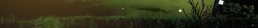
The example below demonstrates a school of fish. Different behavior arises from the interplay between all forces, so you'll have to tweak the numbers to get it right. In this example, Flock.update() has teleport set to True so the boids wrap around the edges instead of turning back. Another thing to remember is to set limit high enough, otherwise the boids will be too constrained and start moving in a straight line.
from nodebox.graphics import *
from nodebox.graphics.physics import Vector, Boid, Flock, Obstacle

flock = Flock(50, x=-50, y=-50, width=700, height=400)
flock.sight(80)

def draw(canvas):
    canvas.clear()
    flock.update(separation=0.4, cohesion=0.6, alignment=0.1, teleport=True)
    for boid in flock:
        push()
        translate(boid.x, boid.y)
        scale(0.5 + boid.depth)
        rotate(boid.heading)
        arrow(0, 0, 15)
        pop()

canvas.size = 600, 300
canvas.run(draw)
References: vergenet.net/~conrad (2007)
Particle system
A particle system is a computer graphics technique to simulate certain fuzzy phenomena which are otherwise very hard to reproduce with conventional rendering techniques: fire, explosions, smoke, moving water, sparks, falling leaves, clouds, fog, snow, dust, meteor tails, hair, fur, grass, or abstract visual effects like glowing trails, magic spells.
Force
A Force causes objects with a mass to accelerate. It acts as a repulsive or attractive dynamic between two particles. A negative strength indicates an attractive force. The closer particles are, the exponentially greater the force will be. The threshold defines a minimum distance to use in calculations – otherwise the force can grow too large (e.g. particles fall outside the canvas before the effect can be perceived) .
force = Force(particle1, particle2, strength=1.0, threshold=100.0)
force.particle1
force.particle2
force.strength
force.threshold
force.apply()
Spring
A Spring exerts attractive resistance when its length changes. It acts as a flexible (but secure) connection between two particles.
spring = Spring(particle1, particle2, length, strength=1.0)
spring.particle1
spring.particle2
spring.strength
spring.length
spring.snapped                             # When True, the spring breaks.
spring.apply()
spring.draw()
Particle
A Particle is an object with a mass that can be subjected to attractive and repulsive forces (unless Particle.fixed is set to True). The object's velocity is an inherent force (e.g. a rocket propeller to escape gravity). A particle can have a life span, which is the number of updates before it disappears. Each System.update(), a particle loses 1 life. Dead particles are not updated or drawn.
particle = Particle(x, y, velocity=(0.0,0.0), mass=10.0, radius=10.0, life=None, fixed=False)
particle.x                                 # Horizontal position.
particle.y                                 # Vertical position.
particle.mass                              # Weight (lighter = greater forces).
particle.radius                            # Used when drawn (radius != mass).
particle.velocity                          # Vector.
particle.life                              # None, or a number.
particle.age                               # 0.0-1.0, if life is defined.
particle.dead                              # True when age=1.0.
particle.fixed                             # Influenced by forces?
particle.draw()
Particles are drawn as circles whose radius diminishes as they age. The Particle.draw() method can of course be overridden with custom behavior. This is what the default method looks like:
class Particle:
    def draw(self, **kwargs):
        r = self.radius * (1 - self.age)
        ellipse(self.x, self.y, r*2, r*2, **kwargs)
System
A System is a collection of particles, particle emitters, forces and springs:
system = System(gravity=(0,0), drag=0.0)
system.particles                           # List of Particle objects.
system.emitters                            # List of Emitter objects.
system.forces                              # List of Force objects.
system.springs                             # List of Spring objects.
system.gravity                             # Global attractive force.
system.drag                                # Global resisting force.
system.dead                                # True if all particles are dead.
system.append() # Particle, Emitter, Force, Spring.
system.force(strength=1.0, threshold=100, source=None, particles=[])
system.dynamics(particle, type=None)
system.update(limit=30)
system.draw()
- System.force() creates a new Force that is applied between each two particles.
The effect this yields (with a repulsive force) is an explosion.
When source is a Particle, applies the force to this particle against all others.
When particles are given, only apply the force to these Particle objects.
The force is applied to particles present in the system, those added later on are not subjected to the force. Be aware that 50 particles wield yield 50 x 50 / 2 = 1250 forces. This has an impact on performance. - System.dynamics() returns a list of forces on the given particle, filtered by type (e.g. type=Spring).
- System.update() updates the location of the particles by applying forces and firing emitters.
Emitter
The Emitter object can be used as a source that shoots particles in a given direction with a given strength. It can be added to a system with System.append().
emitter = Emitter(x, y, angle=0, strength=1.0, spread=10)
emitter.system                             # System the emitter is part of.
emitter.particles                          # Particles fired by the emitter.
emitter.x                                  # Horizontal position.
emitter.y                                  # Vertical position.
emitter.angle                              # Firing direction.
emitter.strength                           # Firing force.
emitter.spread                             # Less spread = shoots straighter.
emitter.append(particle, life=100)
- Emitter.append() adds a Particle (i.e. ammo) to the emitter.
The optional life parameter sets the default lifespan of the particle – dead particles can be reused (e.g. they are fired again) – otherwise the emitter either stops firing or you need to keep adding more and more particles.
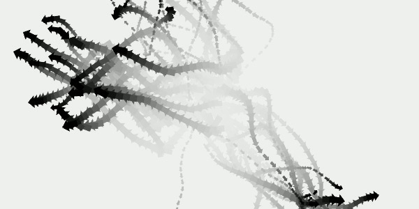
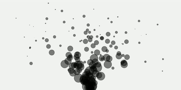
Here is a simple example of a system with an emitter spraying particles:
from nodebox.graphics import *
from nodebox.graphics.physics import System, Emitter, Particle, MASS

e = Emitter(x=300, y=0, angle=90, spread=60, strength=4)
for i in range(100):
    e.append(
        Particle(0, 0,
            life = random(50,250),
            mass = random(10,20),
          radius = MASS)
system = System(gravity=(0,1), drag=0.005)
system.append(e)

def draw(canvas):
    background(1)
    fill(0, 0.5)
    stroke(0, 0.5)
    system.update()
    system.draw()

canvas.size = 600, 300
canvas.run(draw)
References: local.wasp.uwa.edu.au (1998)
Graph
A graph is a data structure consisting of nodes (or vertices) connected by edges. Among other things, graph algorithms are concerned with finding the shortest path between nodes, which could for example represent the road an AI-controlled game character should follow. Or estimating node centrality: which nodes occur more frequently in paths, for example to rank web pages in a network.
Node
The Node object represents an element in the graph. It has a unique id that is drawn as a text label next to the node, unless the optional text parameter is False. Otherwise, the text parameter defines the label color – (0,0,0,1) by default. Optional parameters include: fill, stroke, strokewidth, text, font, fontsize, fontweight to style the node.
node = Node(id="", radius=5, **kwargs)
node.graph                                 # Graph the node is part of.
node.edges                                 # List of Edge objects.
node.links                                 # List of Node objects.
node.id                                    # Unique string or int.
node.x                                     # Horizontal offset.
node.y                                     # Vertical offset.
node.force                                 # Vector, updated by Graph.layout.
node.radius                                # Default: 5
node.fill                                  # Default: None
node.stroke                                # Default: (0,0,0,1)
node.strokewidth                           # Default: 1
node.text                                  # Text object, or None.
node.weight                                # Eigenvector centrality (0.0-1.0).
node.centrality                            # Betweenness centrality (0.0-1.0).
node.flatten(depth=1) # List of linked nodes + self.
node.draw(weighted=False)
node.contains(x, y) # True => (x,y) in radius.
- Node.links.edge(node) yields the Edge connecting this node to the given node.
- Node.draw() draws the node as a circle with the defined radius, fill and stroke.
With weighted=True, a node with a high centrality is marked with a dropshadow.
Node weight and centrality
- Node.centrality indicates the node's betweenness: how often it occurs in shortest paths, as a value between 0.0-1.0. Highly trafficked nodes can be thought of as hubs, landmarks, city centers and so on.
- Node.weight indicates the node's eigenvector centrality: how many nodes are connected to it, as a value between 0.0-1.0. Nodes that (indirectly) connect to high-scoring nodes get a better score themselves. In this case the edge direction plays an important role. Ideally, everyone is pointing at you and you are pointing at no-one - meaning you are at the top of hierarchy.
Edge
The Edge object represents a connection between two nodes. Its weight indicates the importance (not the cost) of the connection. Edges with a higher weight are preferred in shortest paths. Optional parameters include stroke and strokewidth.
edge = Edge(node1, node2, weight=0.0, length=1.0, type=None, **kwargs)
edge.node1                                 # Node (sender).
edge.node2                                 # Node (receiver).
edge.weight                                # Connection strength.
edge.length                                # Length modifier when drawn.
edge.type                                  # None, useful for semantic networks.
edge.stroke                                # Default: (0,0,0,1)
edge.strokewidth                           # Default: 1
edge.draw(weighted=False, directed=False)
edge.draw_arrow(stroke, strokewidth)
- Edge.draw() draws the edge as a line connecting the two nodes.
With weighted=True, a heavier edge will have a thicker strokewidth.
With directed=True, Edge.draw() will call Edge.draw_arrow() to indicate the edge direction (this requires extra calculations).
Graph
The Graph object is a collection of nodes and edges that can be drawn with a given layout. Currently, the only layout available is SPRING, which uses a force-based algorithm in which edges are regarded as springs. The forces are applied to the nodes, pulling them closer together or pushing them further apart.
graph = Graph(layout=SPRING, distance=10.0)
graph.nodes                                # List of Node objects.
graph.edges                                # List of Edge objects.
graph.root                                 # Node or None.
graph.density                              # <0.35 => sparse, >0.65 => dense
graph.distance                             # Overall layout spacing.
graph.layout                               # GraphSpringLayout.
graph.add_node(id, *args, **kwargs, root=False)
graph.add_edge(id1, id2, *args, **kwargs)
graph.remove(node)
graph.remove(edge)
graph.node(id)                             # Returns Node with given id.
graph.edge(id1, id2)                       # Returns Edge for given node id's.
graph.betweenness_centrality()             # Updates Node.centrality.
graph.eigenvector_centrality()             # Updates Node.weight.
graph.shortest_path(node1, node2, heuristic=None, directed=False)
graph.shortest_paths(node, heuristic=None, directed=False)
graph.paths(node1, node2, length=4)
graph.sorted(order=WEIGHT, threshold=0.0)
graph.prune(depth=0)
graph.fringe(depth=0)
graph.split()
graph.copy(nodes=ALL)
graph.update(iterations=10, weight=10, limit=0.5)
graph.draw(weighted=False, directed=False)
- Graph.shortest_path() returns a list of nodes connecting two nodes.
- Graph.shortest_paths() returns a dictionary of nodes linked to shortest path.
With directed=True, edges are only traversable in a single direction.
A heuristic function can be given that takes two node id's and returns an additional cost for movement between the two nodes. - Graph.paths() returns a list of paths <= length connecting the two nodes.
- Graph.sorted() returns a list of nodes sorted by WEIGHT or CENTRALITY.
If the value falls below the given threshold, the node is excluded from the list. - Graph.prune() removes all nodes with less or equal links than depth.
- Graph.fringe() returns a list of leaf nodes.
With depth=0, returns the nodes with only one connection.
With depth=1, returns the nodes with one connection + their connections, etc. - Graph.split() returns a list of unconnected subgraphs.
- Graph.copy() returns a new graph from the given list of nodes.
Graph layout
A GraphLayout object calculates node positions iteratively when GraphLayout.update() is called. Currently, the only available implementation is GraphSpringLayout.
layout = GraphSpringLayout(graph)
layout.graph                               # Graph owner.
layout.iterations                          # Starts at 0, +1 on each update().
layout.bounds                              # (x, y, width, height)-tuple.
layout.k                                   # Force constant   (4.0)
layout.force                               # Force multiplier (0.01)
layout.repulsion                           # Maximum repulsion radius (15)
layout.update(weight=10.0, limit=0.5)      # weight => Edge.weight multiplier.
layout.reset()
layout.copy(graph)
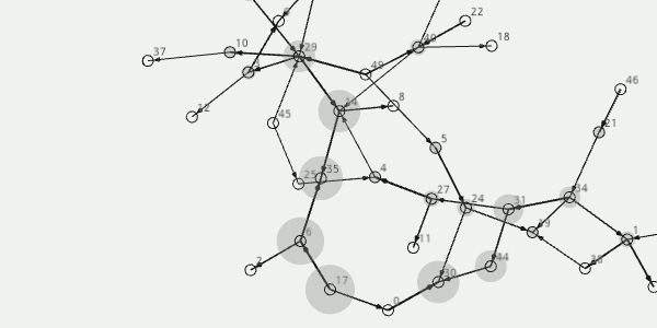
Here is a simple example of a graph with random nodes and edges:
from nodebox.graphics import *
from nodebox.graphics.physics import Node, Edge, Graph

g = Graph()
for i in range(50):
    g.add_node(id=i, stroke=Color(0), strokewidth=1)
for i in range(50):
    node1 = choice(g.nodes)
    node2 = choice(g.nodes)
    g.add_edge(node1.id, node2.id, weight=random(), stroke=Color(0), strokewidth=1)

def draw(canvas):
    background(1)
    translate(250, 250)
    g.draw(weighted=True, directed=True)
    g.update()

canvas.size = 500, 500
canvas.run(draw)
References: NetworkX (2008), Hellesoy & Hoover (2006), Eppstein & Barnes (2005), Brandes (2001)
